by Michael Grogan

In this article we will learn:

* How Bayesian networks function
* How to plot and interpret a directed acrylic graph (DAG)
* How to calculate conditional probabilities with bnlearn

Bayesian networks are quite an intuitive tool when it comes to examining the dependencies between different variables. Specifically, a DAG (or directed acyclic graph) is what allows us to represent the conditional probabilities between a given set of variables.

Using the bnlearn library in Python, let’s take a look at how such analysis can allow us to glean insights on dependencies between different attributes of hotel customers.

Background

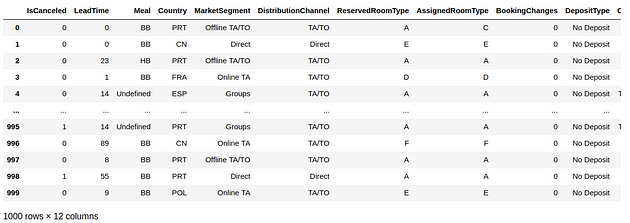
The hotel booking data used in this analysis is from Antonio, Almeida, and Nunes (2019). Taking a dataset of different hotel customer attributes such as whether the customer canceled or not, their country of origin, market segment, etc — 1000 observations from the dataset were drawn at random.

Data Processing and DAG Generation

We will first convert the data into a one-hot data matrix. This function works by auto-detecting the relevant data types and implementing one-hot encoding where necessary:

dfhot, dfnum = bn.df2onehot(df)

Now, we will generate the DAG.

Firstly, the root node is set to IsCanceled, i.e. whether the customer canceled their hotel booking or not. We are setting this as the root node in this case — as we are particularly interested in examining how the different customer attributes affect cancellation behaviour in particular.

Additionally, we also choose to discard certain variables such as Lead Time, as we are primarily interested in analysing categorical features across the dataset and assigning a probability of cancellation based on the different categories included in each feature.

Features that are closely linked with others in the dataset are discarded. For example, ReservedRoomType is closely linked with AssignedRoomType — and thus the decision was taken to discard the former.

DAG = bn.structure_learning.fit(dfnum, methodtype='cl', black_list=['LeadTime', 'Country', 'DistributionChannel','ReservedRoomType'], root_node='IsCanceled', bw_list_method='nodes')G = bn.plot(DAG)

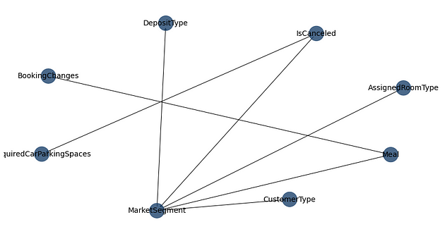
Here is the generated DAG:

As above, we can now see a web-like graph of dependencies between the variables.

For instance, IsCanceled seems to demonstrate a strong conditional probability with MarketSegment and RequiredCarParkingSpaces. In other words, customers from a certain market segment are more likely to cancel than others, and the availability of car parking spaces also seems to be quite influential in whether a customer chooses to cancel or not.

In turn, the MarketSegment variable seems to show a significant dependency with AssignedRoomType and DepositType, among others. For instance, certain market segments might be more amenable to paying a deposit upfront than others, or certain market segments might pay more for a certain room category.

Of course, this is a surface-level analysis in that while a visual of the DAG can show us where dependencies exist between different variables, they cannot explain the nature of those dependencies or why they exist.

From this standpoint, getting an overview of the relationships between different variables before conducting the further analysis can be quite useful.

Further Analysis

After having generated a plot of the DAG in more detail, we can now analyse the parameters in more detail.

A brief look at another example

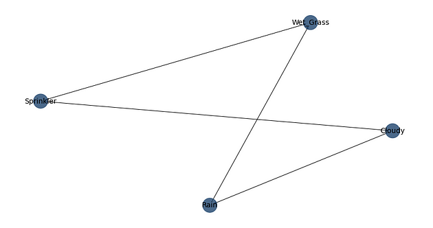
Let’s consider a different example for a moment — the sprinkler example as provided under the bnlearn library.

When analysing the dependencies here, we can see that there exists a relationship between rain and clouds, whether the sprinkler was on or off and the incidence of wet grass.

The CPD (or conditional probability distribution) can be calculated between the variables.

For instance, here is the CPD of the Rain variable that was generated.

[bnlearn] >CPD of Rain:
+---------+--------------------+---------------------+
| Cloudy  | Cloudy(0)          | Cloudy(1)           |
+---------+--------------------+---------------------+
| Rain(0) | 0.6518218623481782 | 0.33695652173913043 |
+---------+--------------------+---------------------+
| Rain(1) | 0.3481781376518219 | 0.6630434782608695  |
+---------+--------------------+---------------------+

If it was cloudy, the probability of not observing rain is at over 65%. The probability of observing rain is at just under 35% under these conditions.

On the other hand, if there were clouds present then the probability of observing rain is at over 66%, with just over a 33% probability of observing no rain.

Back to our hotel example

Now that we have considered a more simplistic example, let’s take a look at some of the CPDs that were generated across the hotel data.

>>> model = bn.parameter_learning.fit(DAG, dfnum)

The probability of seeing a cancellation in its own right is just over 38%.

[bnlearn] >CPD of IsCanceled:
+---------------+-------+
| IsCanceled(0) | 0.611 |
+---------------+-------+
| IsCanceled(1) | 0.389 |
+---------------+-------+

Now, let’s consider the impact of different variables across cancellation probabilities.

Required Car Parking Spaces

We can see that if there are no required car parking spaces available, then the probability of a customer canceling increases significantly.

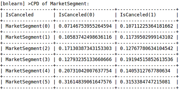
Market Segment

From this CPD, we can also see that certain market segments show a higher cancellation probability than others.

Now, let us suppose that we wish to consider the impact of select combinations of variables on cancellation probabilities.

Let’s take the meal variable as an example. What is the probability of any one customer canceling if the hotel does not cater to a customer’s dietary requirements?

>>> query = bn.inference.fit(model, variables=['IsCanceled'], evidence={'Meal':True})
>>> print(query)
>>> print(query.df)+----+--------------+---------+
|    |   IsCanceled |       p |
+====+==============+=========+
|  0 |            0 | 0.62191 |
+----+--------------+---------+
|  1 |            1 | 0.37809 |
+----+--------------+---------+

Now, what about if we also consider required car parking spaces?

>>> query = bn.inference.fit(model, variables=['IsCanceled'], evidence={'RequiredCarParkingSpaces':True, 'Meal':True})
>>> print(query)
>>> print(query.df)+----+--------------+---------+
|    |   IsCanceled |       p |
+====+==============+=========+
|  0 |            0 | 0.66197 |
+----+--------------+---------+
|  1 |            1 | 0.33803 |
+----+--------------+---------+

We can see that the probability of cancellation falls to just over 33%. When removing the meal variable, the probability is just over 34%. From this standpoint, the analysis indicates that a hotel that has sufficient parking spaces for customers who demand it would be significantly less likely to cancel.

In this way, the bnlearn library is quite useful in both providing a high-level overview of conditional probabilities that exist between variables, as well as a more detailed analysis of the nature of those dependencies.

Many thanks for your time, and any questions or feedback are greatly appreciated. The article was originally published here. You can find more of my data science content at michael-grogan.com.